


The Essence of Machine Learning
Machine learning is suitable for problems where:
- A pattern exists
- We can not pin it down mathematically
- We have data on it
First of all, there has to be a pattern. If there isn't a pattern, the problem is unsolvable, let alone using machine learning to solve it. Second, if a problem can be solve with regular programming (e.g. calculating the Fibonacci number), we normally don't want to solve it with machine learning. It's not because machine learning cannot perform the task, but because doing it the old way would be more efficient. Last but not least, we need to have data in order to do machine learning. Data to machine learning is like petroleum to industrial revolution. Without data, there will be no learning.
Note that sometimes (well most of the times) we don’t know if there’s a pattern or not, but we can still apply machine learning and measure the error. That’s one way to see if there’s a pattern.
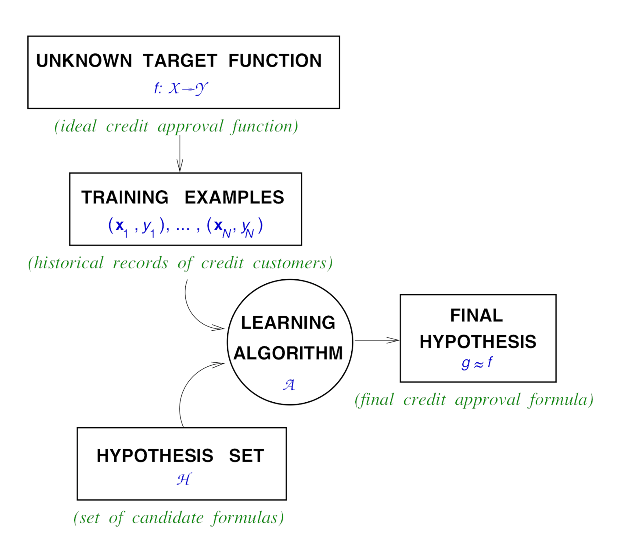
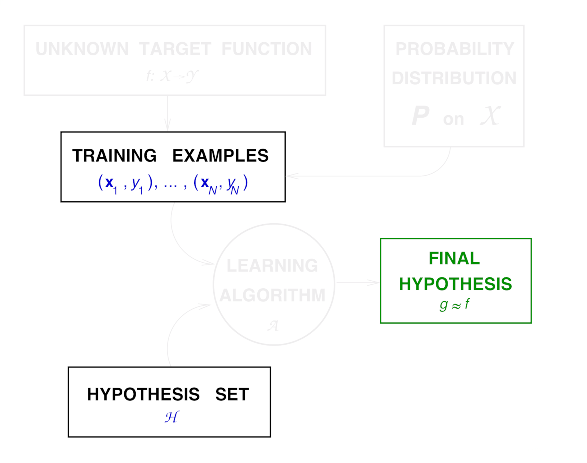
PAC Learning Diagram
PAC stands for probably approximately correct. It is a machine learning framework proposed by Leslie Valiant. In this framework, the learner receives samples and must select a generalization function (called the hypothesis) from a certain class of possible functions. The goal is that, with high probability (the "probably" part), the selected function will have low generalization error (the "approximately correct" part). The learner must be able to learn the concept given any arbitrary approximation ratio, probability of success, or distribution of the samples.
The hypothesis set and learning algorithm together, is called a Learning Model.

Hoeffding's Inequality
In order to discuss the learnability problem, we need to introduce the concept of Hoeffding's Inequality first. Consider flipping a bias coin with the frequency of head being an unknown value . We flip the coin times. The frequency of head in our big samples is . Does the sample frequency say anything about the actual frequency ?
By the definition of Hoeffding's Inequality, is probably close to within an error if we have a large enough set of samples. Formally,
For example, if we have a bias coin with , and flip the coin 10000 times. Hoeffding's Inequality says that the chance of we getting more than 6100 heads or less than 5900 heads () is no more than 0.2707.
Apply Hoeffding's Inequality to The Learning Problem
We will break down this section into three sub-sections:
- The learning problem for a single hypothesis (Testing)
- The learning problem for a hypothesis set (Training)
- The modified Learning Diagram (with Hoeffding's Inequality)
For a single hypothesis (Testing)
Imagine we are picking inputs from an input space wiht probability distribution . We call the sample set .For a hypothesis from the set , we predict the output and compare it with . There are two cases:
- The hypothesis get it right:
- The hypothesis get it wrong:
Now the case where the hypothesis get it right is just like the case where we get a head in flipping a coin. For all the samples , we calculate the frequency of and call it ; we call the unknown frequency , that is,
- In-sample accuracy
- Out-of-sample accuracy
Applying Hoeffding's Inequality
Looking at this equation, on the left hand side, it is the probability of our in-sample error doesn't track the out-of-sample error (a bad event); On the right hand side, it says the probability is less than or equal to a quantity. This quantity is related to the number of samples.
For a hypothesis set (Training)
The statement above applies to a single hypothesis. When we train a model, we first try a hypothesis to see if it fits our samples, and then another, and then another... In essence, we try some hypotheses until one hypothesis turns up that satisfies our pre-determine criteria. This increase the probability of the bad event happening.
Using the notations from before,
Where is the size of the hypothesis set.
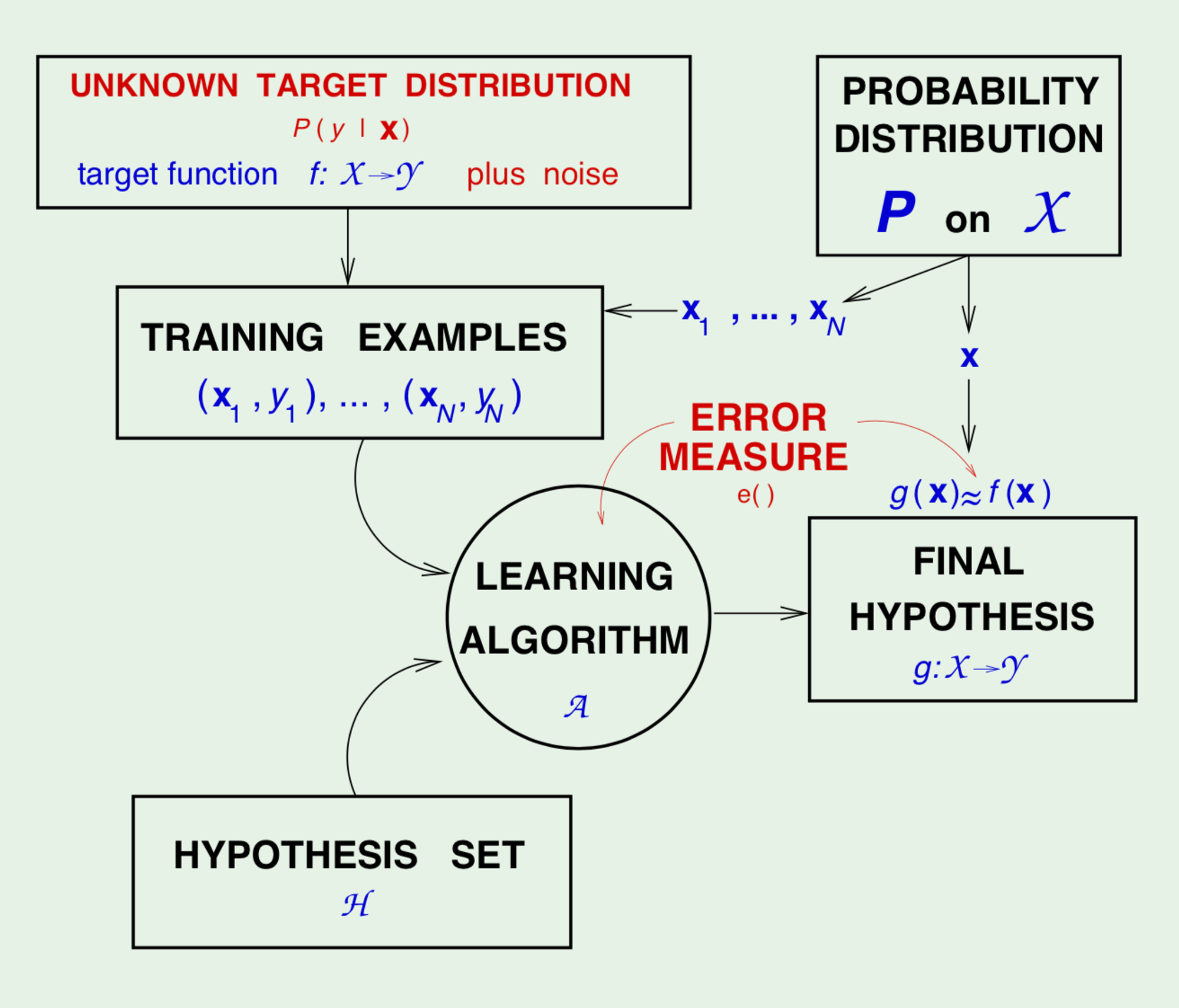
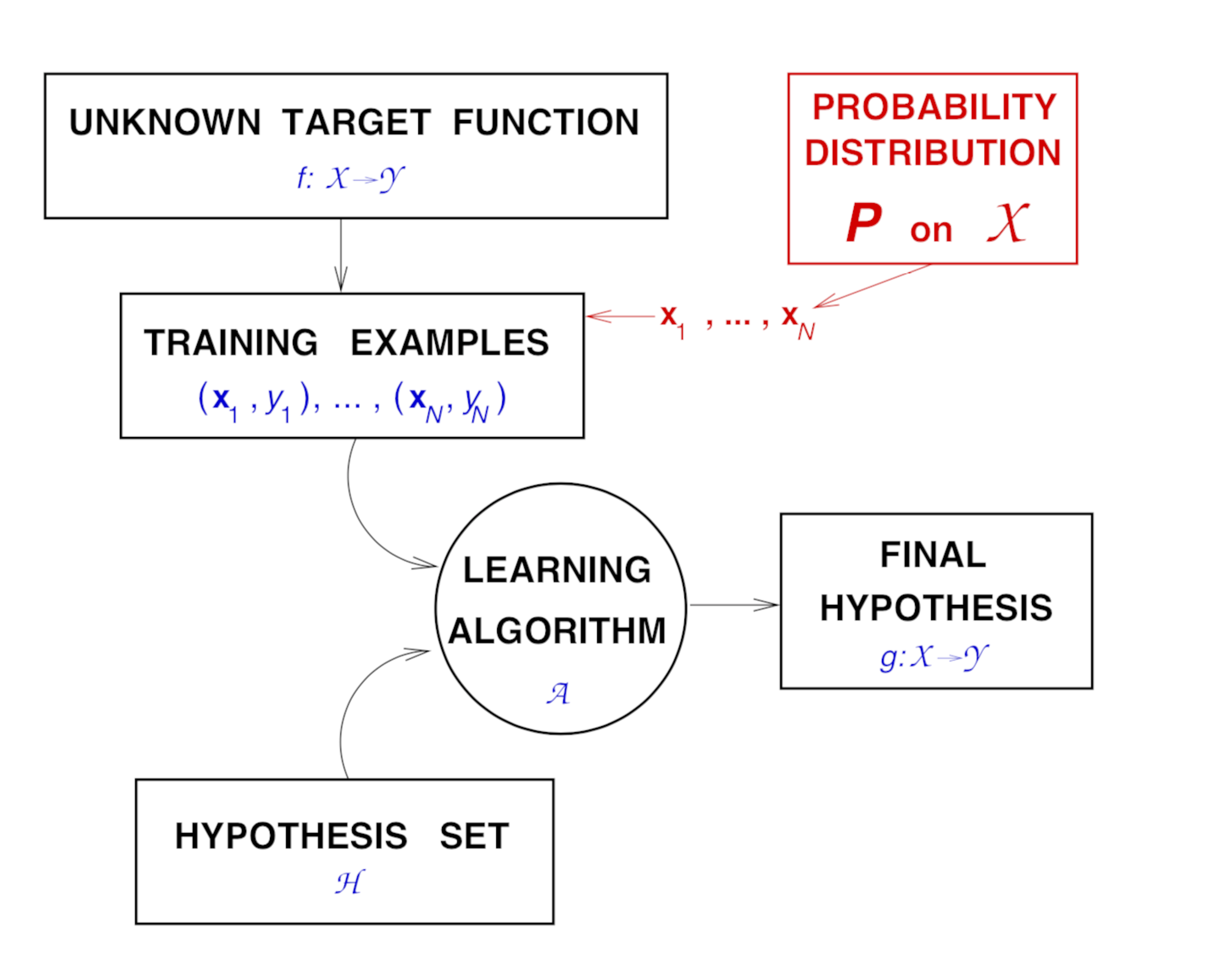
Modified Learning Diagram (with Hoeffding's Inequality)
In this section, we seek to apply Hoeffding's inequality to our PAC learning framework. But looking at the learning diagram from previous section, some pieces are missing, namely the sample space the probability distribution of our samples . We include them here for completeness purpose.

Error Measure
We need an error measure to evaluate the hypotheses. This error measure should be specific to the user case. We make the formal definition of error in this section.
Most of the time, instead of measuring the accuracy, we are more interested in the error. For a binary classification task, the binary error on a specific sample is given by:
The in-sample and out-of-sample error on the entire sample set are:
- In-Sample Error (for )
- Out-of-Sample Error
Noisy Target
There are cases where the target function is not actually a function. For example, credit approval. Two candidates could have the same salary, identical time for residency, etc, yet one got approved while the other one got rejected. This suggests that our target function is not really a function. Because if it were a function, , for any given input , it should have and only have one output .
To accommodate situations like this, instead of , we use target distribution
Any sample pair can now be generated from the joint distribution
Final Learning Diagram
Including error measure and noisy target into our learning diagram, we get its final form
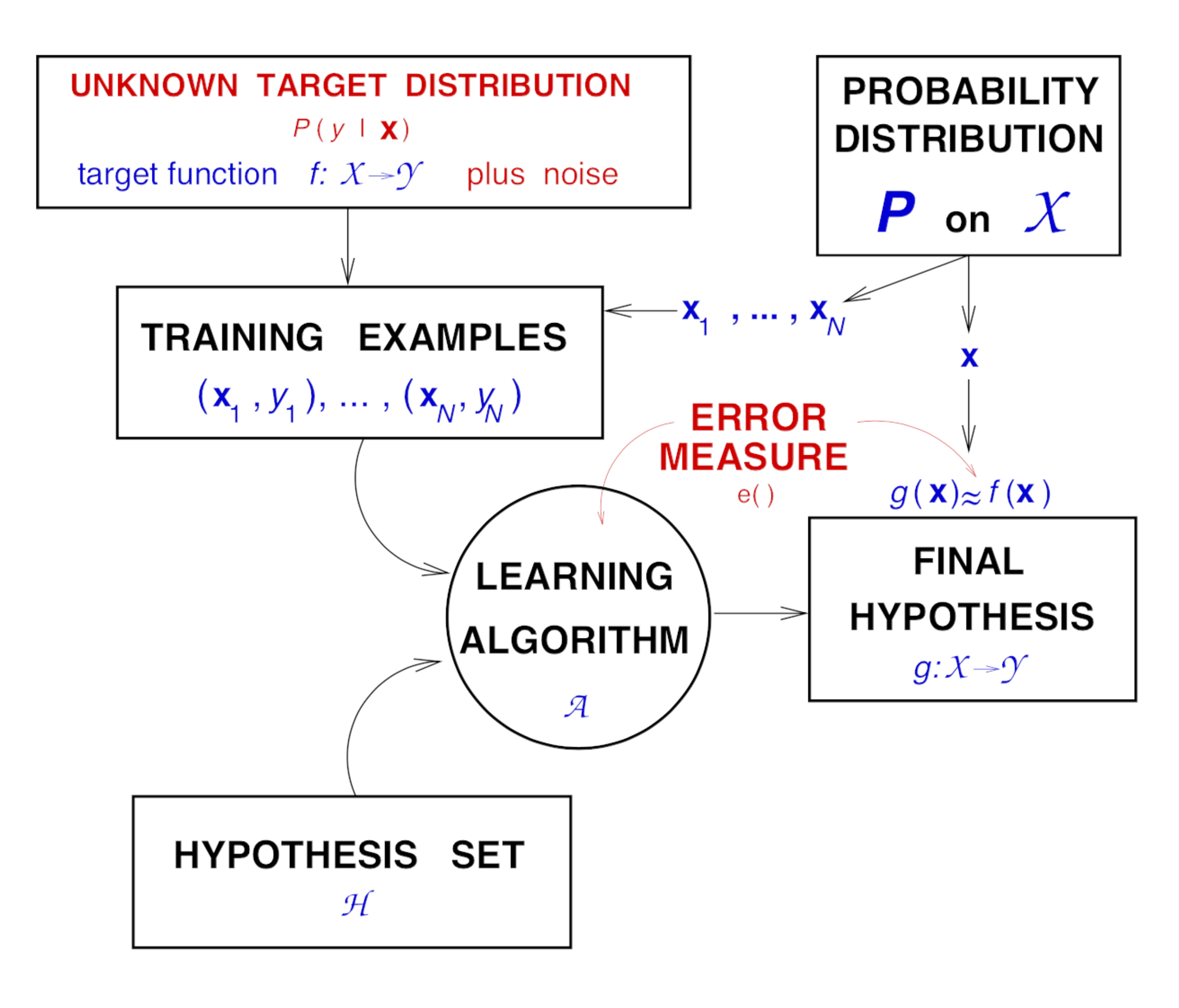
Hoeffding's inequality becomes
Where is the size of the hypothesis set. In this framework, a successful machine learning job comes down to two points:
- Can we make closed enough to ?
- Can we make small enough (close to zero)?
The first point says we should create a dataset that can represent the target data space. The second point corresponds to training a model with the dataset to achieve a low cost error.
VC Theory
Hypotheses vs Dichotomies
Let's take another look on the Hoeffding's Inequality in the training case
Where is the size of the hypothesis set.
But even for a simple hypothesis set like perceptron, the size of the hypothesis set is infinite. Our next step to replace with something more practical.
For a finite sample set
- A hypothesis
- A dichotomy
- Number of hypotheses can be infinite
- Number of dichotomies is at most
Growth Function
Some definitions first. The growth function counts the most dichotomies on any points for a given hypothesis set . If no data set of size can be 'shattered' by a hypothesis set , then is a break point for . Properties of break points:
- For a hypothesis set , if is a break point, is also a break point
- No break point for all
- Any break point is polynomial in
- The existence of a break point suggests learning is feasible
- The value of the break point suggests the samples needed
It turns out that we can use the growth function to replace with some minor modifications to Hoeffding's Inequality. And this is called the Vapnik-Chervonenkis Inequality.
VC Dimension
The VC dimension of a hypothesis set , denoted by , is the largest value of for which . Or, in plain English, VC dimension is the most points can shatter. Referring to the Learning Diagram, VC dimension has a nice property that it only relates to and the samples, which makes it ideal for evaluating a hypothesis set before training.

Examples of VC dimensions:
Hypothesis Set | VC Dimensions |
Positive Rays | 1 |
Positive Intervals | 2 |
d-dimensional Perceptron | d+1 |
In essence, measures the effective number of parameters.
Upper bound on
It can be proved that for a given hypothesis set , . Putting this result and the Vapnik-Chervonenkis Inequality together, we can conclude that is finite will generalize.